Four-Point susceptibility

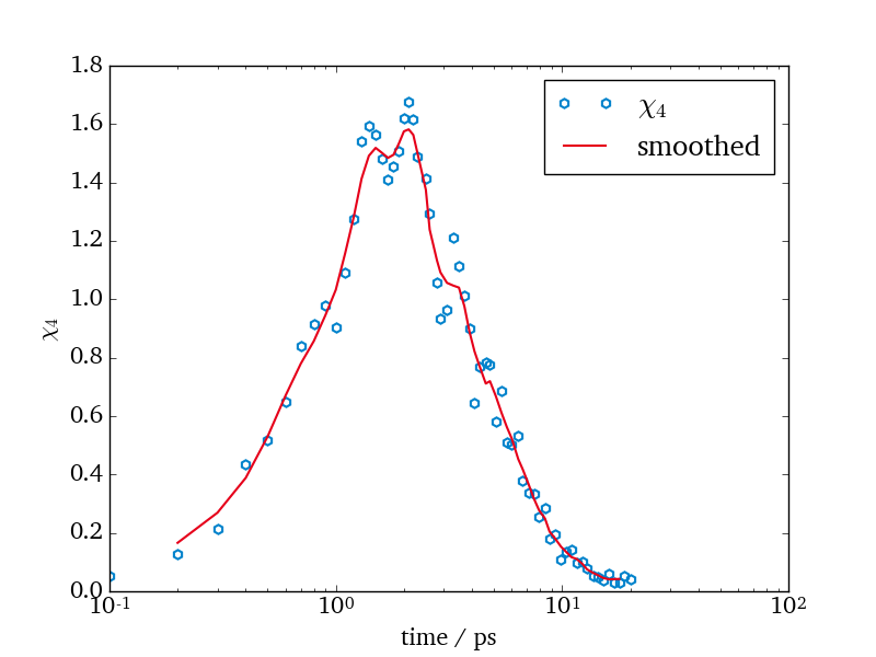
The dynamic four-point susceptibility \(\chi_4(t)\) is a measure for heterogenous dynamics. [Berthier] It can be calculated from the variance of the incoherent intermediate scattering function \(F_q(t)\).

\[\chi_4 (t) = N\cdot\left( \left\langle F_q^2(t) \right\rangle - \left\langle F_q(t) \right\rangle^2 \right)\]

This is astraight forward calculation in mdevaluate. First calculate the ISF without time average and then take the variance along the first axis of this data. Note that this quantity requires good statistics, hence it is adviced to use a small time window and a sufficient number of segments for the analysis. Another way to reduce scatter is to smooth the data with a running mean, calling runningmean() as shown below.

[Berthier]

http://link.aps.org/doi/10.1103/Physics.4.42

Out:

Loading topology: /data/niels/sim/water/bulk/260K/topol.tpr
Loading trajectory: /data/niels/sim/water/bulk/260K/out/traj_full_water1000bulk260.xtc

from functools import partial
import matplotlib.pyplot as plt
import mdevaluate as md
import tudplot

OW = md.open('/data/niels/sim/water/bulk/260K', trajectory='out/*.xtc').subset(atom_name='OW')

t, Fqt = md.correlation.shifted_correlation(
    partial(md.correlation.isf, q=22.7),
    OW,
    average=False,
    window=0.2,
    skip=0.1,
    segments=20
)
chi4 = len(OW[0]) * Fqt.var(axis=0)

tudplot.activate()

plt.plot(t, chi4, 'h', label=r'$\chi_4$')
plt.plot(t[2:-2], md.utils.runningmean(chi4, 5), '-', label='smoothed')

plt.semilogx()
plt.xlabel('time / ps')
plt.ylabel('$\\chi_4$')
plt.legend(loc='best')

Total running time of the script: (0 minutes 0.537 seconds)

Download Python source code: plot_chi4.py

Download IPython notebook: plot_chi4.ipynb